Ishaan Varshney


Confidence Intervals vs Prediction Intervals (in Python)
Context
Statistics is useful because it helps us predict phenonemen. However, whenever we enter the field of predictions we also need to provide a level of uncertainty (or confidence) associated with that estimate.
Let’s explore the idea of uncertainty with an example.
TV advertising -> Sales
This example has been lifted from the book Introduction to Statistical Learning
Data
advertising_data.head()[['TV', 'Sales']]
| TV | Sales | |
|---|---|---|
| 0 | 230.1 | 22.1 |
| 1 | 44.5 | 10.4 |
| 2 | 17.2 | 9.3 |
| 3 | 151.5 | 18.5 |
| 4 | 180.8 | 12.9 |
Regression
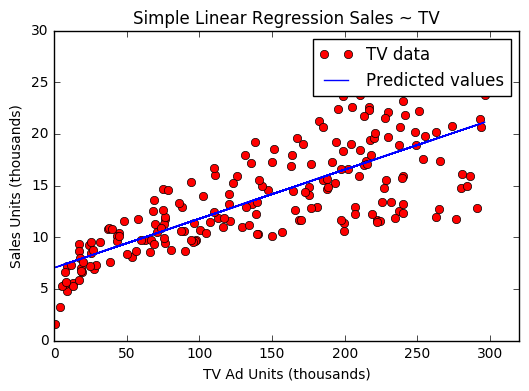
Let’s perform simple linear regresssion with TV advertising being the independant variable
import statsmodels.formula.api as sm
res = sm.ols("Sales ~ TV", advertising_data).fit()
plt.plot(advertising_data["TV"], advertising_data['Sales'], 'ro')
plt.plot(advertising_data["TV"], res.fittedvalues, 'b')
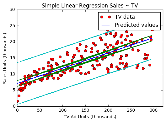
Now let’s plot the confidence and prediction intervals on the historical data.
from statsmodels.stats.outliers_influence import summary_table
st, data, ss2 = summary_table(res, alpha=0.05)
I recommend exploring the output of summary_table as it contains information relating to confidence and prediction intervals. Also the docs for statsmodels are not too helpful in this area.
ci_low = data[:,4]
ci_hi = data[:,5]
pi_low = data[:,6]
pi_hi = data[:,7]


plt.plot(advertising_data["TV"], advertising_data['Sales'], 'ro')
plt.plot(advertising_data["TV"], res.fittedvalues, 'b')
plt.plot(advertising_data["TV"], ci_low, 'g--')
plt.plot(advertising_data["TV"], ci_hi, 'g--')
plt.plot(advertising_data["TV"], pi_low, 'c--')
plt.plot(advertising_data["TV"], pi_hi, 'c--')
Predictions
We can either:
1) predict the average sales of branches that spent 100,000 units on TV advertising
2) predict the sales of one branch that spent 100,000 units on TV adversiting
Depending which of the above we choose to predict, we will have different error bounds as there are differing levels of uncertainty associated with each prediction. However, the bounds for the both cases will centre around the same point. In other words, they will both predict the same value
The bounds associated with (1) average prediction is called the confidence interval. While the bounds around (2) a single point is called the prediction interval.
The bounds for a single point will be greater than the average of those points. There is greater uncertainty associated with the a single prediction because we have to account for irreducible errors. When we take the average of the points we assume that the irrecible errors from all the points will cancel each other out.
At some point, I’ll do a post about irreducible errors in a linear regression to explore this idea further.
Calculating confidence intervals for an exogenous point.
Using our simple linear regression model, let’s predict the Sales when we spend 100 units on TV advertising and the associated CI and PI values.
By hand
$$
CI: \hat{y}\space \pm \space t_{n-2}^\star s\sqrt{\frac{1}{n} + \frac{(x^* - \bar{x})^2}{((n-1)s_x^2)}}
\\
\\
PI: \hat{y}\space \pm \space t_{n-2}^\star s\sqrt{1 + \frac{1}{n} + \frac{(x^* - \bar{x})^2}{((n-1)s_x^2)}}
$$
where s is the residual standard error
Calulating the confidence intervals from scratch we get:
from scipy import stats

x = 1/len(advertising_data) + (pow(100-tv_bar,2)/((len(advertising_data)-1)*pow(tv_s,2)))
conf_low = pred - stats.t.ppf(1-0.025, 198) * se*pow(x, 0.5)
conf_hi = pred + stats.t.ppf(1-0.025, 198) * se*pow(x, 0.5)
Output
>> print(conf_low, conf_hi)
>> [ 11.26583257] [ 12.30668261]
Calculating the prediction intervals from scratch, we get:
rss = sum([pow(advertising_data["TV"], 2) for x in res.resid])
rse = pow(rss/(len(advertising_data['Sales'])-2), 0.5)
RSE can be thought of as the standard deviation of the residuals.
from scipy import stats
# using the above formula
x = 1 + 1/len(advertising_data) +
    (pow(100-tv_bar,2)/((len(advertising_data)-1)*pow(tv_s,2)))
pred_low = pred - stats.t.ppf(1-0.025, 198) * se*pow(x, 0.5)
pred_hi = pred + stats.t.ppf(1-0.025, 198) * se*pow(x, 0.5)
Output
>> print(conf_low, conf_hi)
>> [ 5.31828015] [ 18.25423503]
Alternatively one can find the prediction interval bounds by:
from statsmodels.sandbox.regression.predstd import wls_prediction_std

pred = res.predict(exog={"TV":100})
_ pred_low, pred_high = wls_prediction_std(res, exog=[1,100], weights=1)

# However we get slightly different results. Not 100% that it's just rounding error]

Output:
[ 5.33925132] [ 18.23326387]
Takeaways
Confidence intervals can be thought of as the error bounds associated with average of several points at that value.
Prediction intervals are the error bounds for the single point.
Confidence intervals are narrower than prediciton intervals because the average of the points cancels out the irreducible error.
Python’s
statsmodelslibrary’s documentation and interface is not as clean as the R language’s. We should work towards bettering it.